The noise object

The figure above shows how the noise is processed in the circuit processor. The noise is defined separately in a class object. When called, it takes parameters from the processor (like operators or coefficients), modifies them and returns them to the processor. However, this design has a drawback. Since the Hamiltonian saved in the circuitprocessor is a list of operators and their amplitudes. It restricts the form of the noise, for instance, it is not possible to create noise with coefficient represented by string based functions.
To allow more diversity in the noise we can use the newly implemented class qutip.QobjEvo. The QobjEvo consists of evolution elements qutip.EvoElement, which contains the information of the Hamiltonian operators, the coefficients and the time list. The advantage is that it allows different types of time-dependent coefficients for different EvoElement.
With this the noise can be defined independently from the circuit processor, for instance:
- Decoherence noise: defined by the collapse operators, with optional parameters like time-dependent coefficients or target qubits.
- Control amplitude noise: defined by the noisy coefficients. It can be added to the existing Hamiltonians in the processor or to totally different operators.
- When calculating the evolution, the processor first creates its own QobjEvo. Usually, it just contains the desired unitary evolution.
- It will then find all the noise objects saved in it and call the corresponding methods to get the QobjEvo representing these noisy dynamics.
- For each noise object, the necessary information is passed from the processor to it (like the Hamiltonians, the coefficients or the parameters defined in the processor). The additional dynamics are calculated in the noise object and returned the processor either in another QobjEvo, or in a list of Qobjs (For collapse operators, we don't want to add all the constant collapse into one time-independent operator, so we use a list).
- The processor then combines its own QobjEvo with those from the noise object and give them to the solver.

The advantage of this design is its flexibility and compatibility. Different types of coefficients, as long as they are allowed in the QuTiP solver, can be used to construct the noise object. We can also easily implement a framework for user-defined noise classes. The limitation is that if NumPy Array is used as coefficients, it has to have the same length as tlist, so it is difficult to add e.g. noise with smaller time interval than tlist.
An example with jupyter notebook can be found at https://github.com/BoxiLi/Exaples_GSoC/blob/master/CircuitNoise.ipynb
Comments
Post a Comment