Demo for the circuit processor and the effect of noise for simple quantum gates
Example for spin chain and cqed model
%matplotlib inline
from qutip import *
from qutip.qip.models.spinchain import *
from qutip.qip.models.circuitprocessor import *
from qutip.qip.models.cqed import *
N = 3
qc = QubitCircuit(N)
qc.add_gate("CNOT", targets=[0], controls=[2])
Spinchain model
This module takes a quantum circuit and find a pulse sequence generating the circuit with the Hamiltonian realsized by the spinchain model.
It first resolves the gate into the following gates : "GLOBALPHASE", "ISWAP", "RX", "RZ" and then genearte a time-dependent hamitonian sequence consisting of $\sigma_{x}$, $\sigma_{z}$ and $\sigma_{x}\sigma_{x}+\sigma_{y}\sigma_{y}$
lsc = LinearSpinChain(N, correct_global_phase=True)

# create pulse sequences
U_list = lsc.run(qc)
# resolved gates from "ISWAP", "RX", "RZ"
lsc.qc2.gates
lsc.plot_pulses();

CQED model
The state is represented by a resonator mode of $N_{res}$ levels and qubits states of $N$ levels. The availabel Hamitonian is $\sigma_x$, $\sigma_z$ and the qubit-cavity interaction $a^\dagger \sigma^- + a \sigma^+$.
qc = QubitCircuit(N)
qc.add_gate("CNOT", targets=[0], controls=[2])
# qc.add_gate("SWAP", targets=[0,2])
cqed = DispersivecQED(3)
U_list = cqed.run(qc)
Resolved gate sequence from "ISWAP", "RX", "RZ". It is a bit different compared to linear spin chain because of boundary conditions
cqed.qc2.gates
cqed.plot_pulses();

from qutip import *
import numpy as np
import matplotlib.pyplot as plt
from numpy.random import normal as gauss
pi = np.pi
Hadamard gate can be generated by Hamiltonian $\sigma_y$ and a $\sigma_z$ for time $t_1$ and $t_2$
$u = \exp[-i\sigma_z t_2]\cdot\exp[-i\sigma_y t_1]$
H1 = sigmay()
H2 = sigmaz()
t1 = 3./4.*pi
t2 = 1./2.*pi
up = basis(2,0)
This can be proved by explicit calculation
u1 = (-1.j * t1 * H1).expm()
u2 = (-1.j * t2 * H2).expm()
u = u2*u1
u
Now we use mesolve to calculate the state evolution under these two pulses and vary $t_1$ for Hamiltonian $\sigma_z$. We start from $|{\uparrow}>$ and should get $|+>$ if $t=t_1$
def noisy_Hadamard(t1):
    iter_num = 50

    rho0 = basis(2,0)
    tlist = np.linspace(0,t1,iter_num)
    H = [[H1, np.ones(iter_num)]]
    result = mesolve(H, rho0, tlist)

    rho1 = result.states[-1]
    tlist = np.linspace(0,t2-0.03,iter_num)
    H = [[H2, np.ones(iter_num)]]
    result = mesolve(H, rho1, tlist)

    return result.states[-1]
t1_line = np.linspace(0.8*t1,1.2*t1,30)
plus = (basis(2,0)+basis(2,1)).unit()
F_line = list(map(lambda t1: fidelity(noisy_Hadamard(t1), plus), t1_line))
We plot the fidelity as a function of $t/t_1$
plt.plot(t1_line/t1, F_line)
plt.xlabel("$t'/t_1$")
plt.ylabel("Fidelity");

CNOT gate
We do the same for CNOT gate. We assume here that all the single qubit operations are perfect and only the two qubit interaction is noisy.
t = pi/8
# two qubits interaction
H = (tensor(sigmax(),identity(2)) + tensor(identity(2),sigmax()))**2
u = (-1.j*t*H).expm()
snot12 = tensor(snot(),snot())
snot1 = tensor(snot(),identity(2))
snot2 = tensor(identity(2),snot())
snot1* u * snot12 * tensor(rz(-pi/2),rz(-pi/2)) * snot2
def noisy_CNOT(t):
    iter_num = 50
    rho = tensor(basis(2,1),basis(2,0))
    rho = snot12 * tensor(rz(-pi/2),rz(-pi/2)) * snot2 * rho
    tlist = np.linspace(0,t,iter_num)
    result = mesolve([[H, np.ones(iter_num)]], rho, tlist)
    return snot1* result.states[-1]
We start from the $|10>$ state and should get $|11>$ state if the operation is perfect
t_line = np.linspace(0.8*t,1.2*t,30)
correct_end_state = tensor(basis(2,1),basis(2,1))
F_line = list(map(lambda t: fidelity(noisy_CNOT(t), correct_end_state), t_line))
plt.plot(t_line/t, F_line)
plt.xlabel("$t'/t$")
plt.ylabel("Fidelity");

Comments
Post a Comment